Introduction

This tutorial demonstrates the usage of NiHu for solving an exterior acoustic radiation problem in 3D by means of a collocational type boundary element method (BEM). It is well known that the standard BEM formulation, when applied to an exterior radiation problem, does not have a unique solution at the eigenfrequencies of the dual interior problem. This tutorial presents how two mitigation methods,

the CHIEF method
and the Burton Miller formalism

are applied to handle the problem.

If you are familiar with the CHIEF and Burton Miller formalisms, you should be able to implement the C++ code based on the previous tutorial A Galerkin BEM for the Helmholtz equation. However, it is worth reading this tutorial, because it will demonstrate how the complete solution is assembled in NiHu for both approaches.

Theory

The eigenfrequency problem

The Helmholtz boundary integral equation

\( \displaystyle \frac{1}{2} p({\bf x}) = \left(\mathcal{M}p\right)_S({\bf x}) - \left(\mathcal{L}q\right)_S({\bf x}), \quad \bf{x} \in S \)

when applied to exterior radiation or scattering problems, does not have a unique solution at the eigenfrequencies of the dual interior problem. It can be shown that the interior mode shapes \( p^*_k({\bf y}) \) and their normal derivatives \( q^*_k({\bf y}) = \partial p^*_k({\bf y}) / \partial n_{\bf y} \) satisfy the boundary integral equation, although, obviously, they have no phyiscal relation to the exterior problem.

The two discussed solution methods mitigate the problem by extending the integral equation by other equations that are not satisfied by the modal solution.

The CHIEF method

The CHIEF method (the name comes from Combined Helmholtz Integral Equation Formalism) utilises the fact that the mode shapes \( p^*_k({\bf y}) \) do not satisfy the Helmholtz integral with source point \( {\bf x} \) inside the interior volume, if the source point coincides with a nodal location of the mode shape. Therefore, the boundary integral equation is extended by a set of additional equations as follows:

\( \displaystyle \frac{1}{2} p({\bf x}) = \left(\mathcal{M}p\right)_S({\bf x}) - \left(\mathcal{L}q\right)_S({\bf x}), \quad {\bf x} \in S, \\ \displaystyle \phantom{\frac{p({\bf x})}{2}} 0 = \left(\mathcal{M}p\right)_S(\tilde{\bf x}_l) - \left(\mathcal{L}q\right)_S(\tilde{\bf x}_l), \quad \tilde{\bf x}_l \in V^{\text{interior}}, \quad l = 1 \dots K \)

Theoretically, one additional equation would be enough to exclude the fictitious solution. However, as it is difficult to estimate where the nodal locations of the interior problem are, the method is usually applied by selecting a number of randomly chosen interior points \( \tilde{\bf x}_l \).

After discretisation, the following overdetermined linear system of equations is to be solved:

\( \displaystyle \left[ \begin{matrix} {\bf M} - {\bf I}/2 \\ {\bf M}' \end{matrix} \right] {\bf p} = \left[ \begin{matrix} {\bf L} \\ {\bf L}' \end{matrix} \right] {\bf q} \)

where

\( \displaystyle L_{ij} = \left< \delta_{{\bf x}_i}, \left(\mathcal{L} w_j\right)_S \right>_S, \quad \displaystyle M_{ij} = \left< \delta_{{\bf x}_i}, \left(\mathcal{M} w_j\right)_S \right>_S \\ \)

are the conventional system matrices ( \(w_j\) denotes the weighting shape function on the surface) of a collocational BEM, and

\( \displaystyle L'_{lj} = \left< \delta_{\tilde{\bf x}_l}, \left(\mathcal{L} w_j\right)_S \right>_S, \quad \displaystyle M'_{lj} = \left< \delta_{\tilde{\bf x}_l}, \left(\mathcal{M} w_j\right)_S \right>_S \)

are the additional matrices originating from the discretised CHIEF equations.

The Burton and Miller Formalism

The Burton and Miller method searches for the solution of the original boundary integral equation and its normal derivative with respect to the normal at \( {\bf x} \):

\( \displaystyle \frac{1}{2} p({\bf x}) = \left(\mathcal{M}p\right)_S({\bf x}) - \left(\mathcal{L}q\right)_S({\bf x}), \quad {\bf x} \in S, \\ \displaystyle \frac{1}{2} q({\bf x}) = \left(\mathcal{N}p\right)_S({\bf x}) - \left(\mathcal{M}^{\mathrm{T}}q\right)_S({\bf x}), \quad {\bf x} \in S \)

where

\( \displaystyle \left(\mathcal{M}^{\mathrm{T}}q\right)_S({\bf x}) = \frac{\partial}{\partial n_{\bf x}}\int_S G({\bf x}, {\bf y}) q({\bf y})\mathrm{d}S_{\bf y} \)

is the transpose of \( \left(\mathcal{M}q\right)({\bf x})\), as differentiation is performed with respect to the variable \( {\bf x} \), and the arising

\( \displaystyle \left(\mathcal{N}p\right)_S({\bf x}) = \frac{\partial}{\partial n_{\bf x}}\int_S \frac{\partial}{\partial n_{\bf y}} G({\bf x}, {\bf y}) p({\bf y})\mathrm{d}S_{\bf y} \)

is operator becomes hypersingular.

The differentiated equation suffers from the problem of fictitious eigenfrequencies too. However, as the eigenfrequencies and mode shapes of the original and differentiated equations never coincide, the simultaneous solution is unique. This solution is found by solving the superposition of the two equations using an appropriate coupling constant \( \alpha \)

\( \displaystyle \left(\left[\mathcal{M} - \frac{1}{2}\mathcal{I} + \alpha \mathcal{N} \right]p\right)_S({\bf x}) = \left(\left[\mathcal{L} + \alpha \mathcal{M}^{\mathrm{T}} + \alpha \frac{1}{2} \mathcal{I}\right] q\right)_S({\bf x}), \quad {\bf x} \in S \)

The collocational discretisation of the above equation is straightforward. However, we should take into consideration that the hypersingular operator's kernel has an \( O(1/r^3) \) type singularity, and needs special treatment. This topic is discussed in details in the tutorial Customising singular integrals.

Program structure

We are going to implement a Matlab-C++ NiHu application, where

the C++ executable is responsible for assembling the system matrices from the boundary surface mesh and the CHIEF points,
the Matlab part defines the meshes, calls the C++ executable, solves the systems of equations, and compares the solutions by quantifying their errors.

The C++ code

The C++ code is going to be called from Matlab as

[L, M, Lchief, Mchief, Mtrans, N] = helmholtz_bem_3d_fict(
    surf_nodes, surf_elements, chief_nodes, chief_elements, wave_number);

Note: The CHIEF points are defined as element centres of a NiHu mesh for convenience. With this choice, the applied discretisation formalism is identical to that of a radiation integral in tutorial Rayleigh integral.; The computed system matrices M and Mtrans will contain the discretised identity operator too, as required by the conventional and Burton-Miller formalisms.

Header and mesh creation

The header of our C++ source file includes the necessary header files and defines some basic types for convenience. We further include library/helmholtz_singular_integrals.hpp that defines the specialised singular integrals of the Helmholtz kernel for constant triangles.

#include <mex.h>
 
#include "core/weighted_residual.hpp"
#include "util/mex_matrix.hpp"
#include "library/helmholtz_3d.hpp"
 
typedef NiHu::mex::real_matrix<double> dMatrix;
typedef NiHu::mex::complex_matrix<double> cMatrix;

Two meshes will be created:

One for the radiator surface (surf_mesh) that contains only triangular elements
One for the CHIEF points (chief_mesh) that contains only quadrangle elements
Note
Only the element centres of the CHIEF point mesh are important

dMatrix

surf_nodes(rhs[0]), surf_elem(rhs[1]),

chief_nodes(rhs[2]), chief_elem(rhs[3]);

auto surf_mesh = NiHu::create_mesh(surf_nodes, surf_elem, NiHu::tria_1_tag(), NiHu::quad_1_tag());

auto chief_mesh = NiHu::create_mesh(chief_nodes, chief_elem, NiHu::quad_1_tag());

Definition of function spaces

Next, we create the discretised function spaces of our mesh. The definitions are straightforward, as only constant triangular boundary elements are dealt with. For the definition of the CHIEF mesh, we immediately apply the dirac view.

auto const &surf_sp = NiHu::constant_view(surf_mesh);

auto const &chief_sp = NiHu::dirac(NiHu::constant_view(chief_mesh));

The number of degrees of freedom on the radiating surface \( S \) and in the field mesh \( F \) are denoted by \( n \) and \( m \), respectively. After the function spaces are built, the number of DOFs are known, and the memory for the system matrices can be preallocated. The surface system matrices \( \mathbf{L} \), \( \mathbf{M} \), \( \mathbf{M}_\mathrm{transpose} \) and \( \mathbf{N} \) are of size \( n \times n \), whereas the matrices describing the CHIEF equations \( \mathbf{M}' \) and \( \mathbf{L}' \) are of size \( m \times n \). The six system matrices are preallocated by means of the following lines of code.

    size_t n = surf_sp.get_num_dofs();
    size_t m = chief_sp.get_num_dofs();
    cMatrix
        L_surf(n, n, lhs[0]), M_surf(n, n, lhs[1]),
        L_chief(m, n, lhs[2]), M_chief(m, n, lhs[3]),
        Mt_surf(n, n, lhs[4]), N_surf(n, n, lhs[5]);

Integral operators and their evaluation

In the next steps, the five integral operators \( \mathcal{L} \), \( \mathcal{M} \), \( \mathcal{M}^\mathrm{T} \), \( \mathcal{N} \) and \( \mathcal{I} \) are defined. Since the kernel functions depend on the wave number \( k \), which is passed as the fifth right hand side parameter of the mex function, the integral operators are created as follows.

    double k = *mxGetPr(rhs[4]);
    auto I = NiHu::identity_integral_operator();
    auto L = NiHu::create_integral_operator(NiHu::helmholtz_3d_SLP_kernel<double>(k));
    auto M = NiHu::create_integral_operator(NiHu::helmholtz_3d_DLP_kernel<double>(k));
    auto Mt = NiHu::create_integral_operator(NiHu::helmholtz_3d_DLPt_kernel<double>(k));
    auto N = NiHu::create_integral_operator(NiHu::helmholtz_3d_HSP_kernel<double>(k));

Finally, the system matrices are obtained by the evaluation of the integral operators on the function spaces defined above. Note that as a collocational formalism is applied, the Dirac-view of the test function spaces is taken for the boundary integrals.

    // conventional equations
    L_surf << dirac(surf_sp) * L[surf_sp];
    M_surf << dirac(surf_sp) * M[surf_sp]  +  dirac(surf_sp) * (-.5*I)[surf_sp];
    // CHIEF equations
    L_chief << chief_sp * L[surf_sp];
    M_chief << chief_sp * M[surf_sp];
    // Burton-Miller equations
    mexPrintf("Integrating transposed kernel\n");
    Mt_surf  << dirac(surf_sp) * Mt[surf_sp] +  dirac(surf_sp) * (.5*I)[surf_sp];
    mexPrintf("Integrating hypersingular kernel\n");
    N_surf  << dirac(surf_sp) * N[surf_sp];

Note: It should be realised that the evaluation of matrices M_surf and Mt_surf contain the evaluation of two integral operators, \( \mathcal{M} \) and \( \mathcal{I} \), or \( \mathcal{M}^{\mathrm{T}} \) and \( \mathcal{I} \) and stores the summed results.

The Matlab code

The example creates a sphere surface of radius \( R = 1\,\mathrm{m} \) centred at the origin, consisting of triangular elements only. The CHIEF points are located on the surface of a cube, shifted from the origin.

The Neumann boundary conditions are defined by a point source located at the point \( \mathbf{x}_0 \). By this definition the geometry is considered transparent, and the resulting acoustic fields on \( S \) are obtained as the acoustic field of the point source.

The compiled mex file can be called from Matlab, as demonstrated in the example below:

%// sphere radiator with radius R = 1, divided into 6 elements along the radius.
radiator = quad2tria(create_sphere_boundary(1, 6));
%// CHIEF-points: element centers of cube boundary
chief_points = create_brick_boundary(.4, 5);
 
%// extract the mesh description matrices
[r_nodes, r_elem] = extract_core_mesh(radiator);
[c_nodes, c_elem] = extract_core_mesh(chief_points);
 
%// call C++ code at wave number k \approx pi
k = pi + 1.2e-2;
[Ls, Ms, Lc, Mc, Mts, Ns] =...
    helmholtz_bem_3d_fict(r_nodes, r_elem, c_nodes, c_elem, k);
 
%// define the incident velocity field and analytical solutions
x0 = [0 0 0];
[r_cent, r_norm] = centnorm(radiator);
[ps_ana, qs_ana] = incident('point', x0, r_cent, r_norm, k);
 
%// acoustic pressure on the surface and in the field points
ps_conv = Ms \ (Ls * qs_ana);               %// conventional
ps_chief = [Ms; Mc] \ ([Ls; Lc] * qs_ana);  %// CHIEF
coup = -1i/k;   %// coupling constant
ps_bm = (Ms + coup * Ns) \ (Ls * qs_ana + coup * Mts * qs_ana);
 
% // calculate errors
ps_conv_err = abs(ps_conv./ps_ana - 1);     %// conventional
ps_chief_err = abs(ps_chief./ps_ana - 1);   %// CHIEF
ps_bm_err = abs(ps_bm./ps_ana - 1);         %// BM
 
% // plot results
figure;
 
plot_mesh(radiator, log10(ps_conv_err));
text(0,1.3,0, 'Conventional', 'HorizontalAlignment', 'center');
plot_mesh(translate_mesh(radiator, [2.3 0 0]), log10(ps_chief_err));
text(2.3,1.3,0, 'CHIEF', 'HorizontalAlignment', 'center');
plot_mesh(translate_mesh(radiator, [2*2.3 0 0]), log10(ps_bm_err));
text(2*2.3,1.3,0, 'Burton-Miller', 'HorizontalAlignment', 'center');
err_tot = [ps_conv_err; ps_chief_err; ps_bm_err];
shading flat; caxis(log10([min(err_tot) max(err_tot)]));
view(2);
c = colorbar('SouthOutside');
xlabel(c, 'Log 10 error of solution');
 
%// display error information
fprintf('Conventional  log10 error: % .3f \n', log10(mean(ps_conv_err)));
fprintf('CHIEF         log10 error: % .3f \n', log10(mean(ps_chief_err)));
fprintf('Burton-Miller log10 error: % .3f \n', log10(mean(ps_bm_err)));

The generated plot looks like

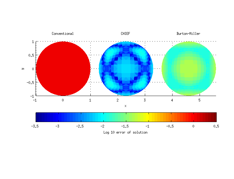
And the resulting errors read as

Conventional  log10 error:  0.025 
CHIEF         log10 error: -2.344 
Burton-Miller log10 error: -1.680

The full codes of this tutorial are available here:

C++ code: tutorial/helmholtz_bem_3d_fict.mex.cpp
Matlab code: tutorial/helmholtz_bem_3d_fict_test.m

Table of Contents